Hash Join

Hash Join

• Micro-topic: Basics (Page 712)
• Micro-topic: Figure 15.9 Hash partitioning of relations. (Page 713)
• Micro-topic: Figure 15.10 Hash join. (Page 714)
• Micro-topic: Recursive Partitioning (Page 714)
• Micro-topic: Handling of Overflows (Page 715)
• Micro-topic: Cost of Hash Join (Page 715)

Basics

Hash join is an efficient algorithm to implement natural joins and equi-joins. It leverages a hash function to partition tuples of both relations, improving performance.

Core Idea:

• Partition tuples of each relation into sets that have the same hash value on the join attributes.
• If an r tuple and an s tuple satisfy the join condition, they have the same value for the join attributes.
• Thus if that value of join attributes, is hashed to some value i, then r tuple must be in $r_i$, and s tuple must be in $s_i$.
• Therefore, r tuples in $r_i$ need to be compared only with s tuples in $s_i$.

Assumptions:

• h: A hash function mapping JoinAttrs values to {0, 1, …, $n_h$}, where JoinAttrs are the common attributes of r and s.
• $r_0,r_1,...,r_{n_h}$: Partitions of r tuples, initially empty. Each tuple $t_r\in r$ is put in partition $r_i$, where i = h($t_r$[JoinAttrs]).
• $s_0,s_1,...,s_{n_h}$: Partitions of s tuples, initially empty. Each tuple $t_s\in s$ is put in partition $s_i$, where i = h($t_s$[JoinAttrs]).

Hash Function Properties:

The hash function h should possess properties of randomness and uniformity.

Figure 15.9: Hash Partitioning of Relations.

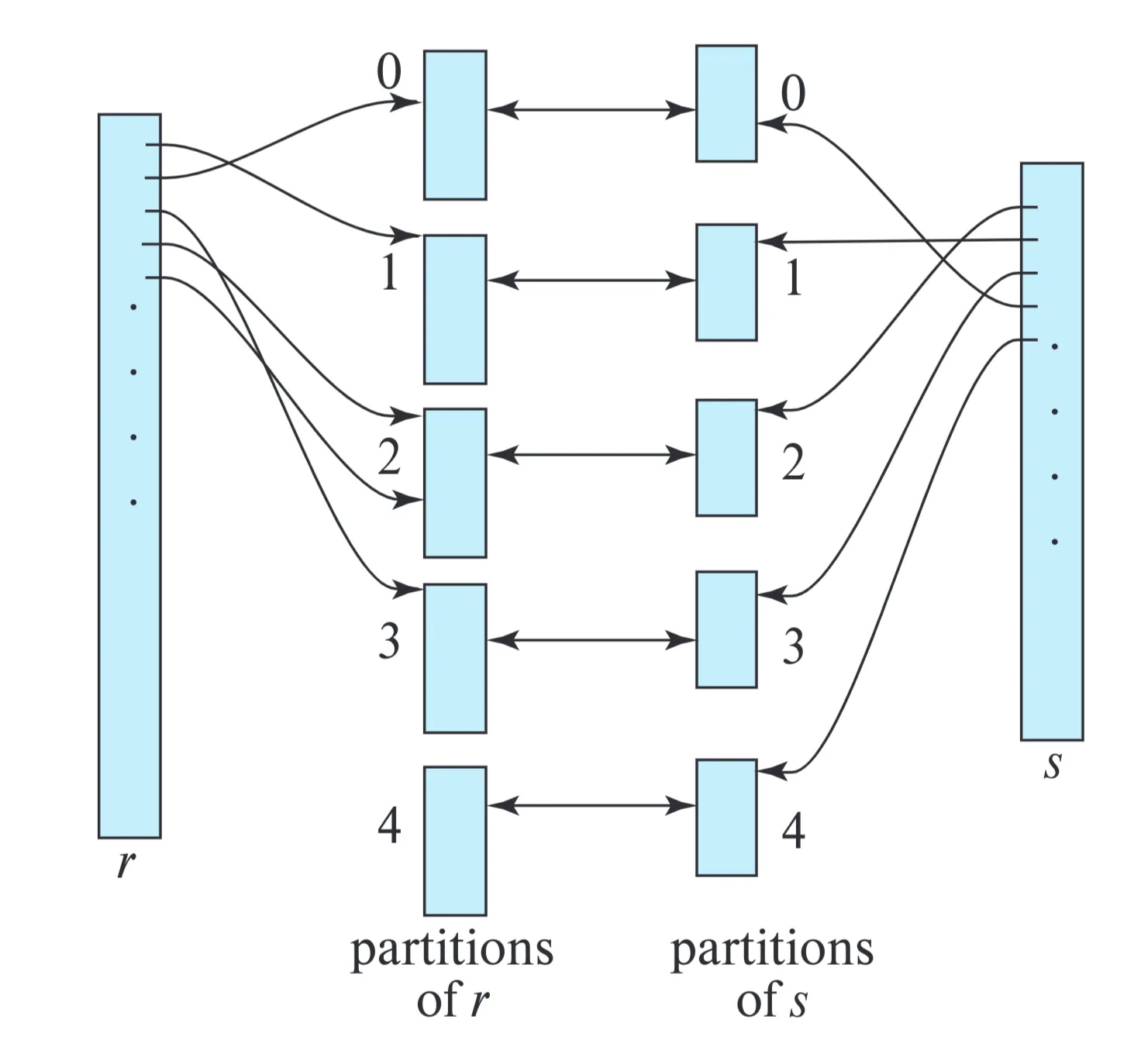
Database System Concepts 7, p.713

Illustrates visually how relations r and s are partitioned using the hash function h. Each partition is shown as a bucket.

Figure 15.10: Hash Join.

Provides the complete pseudocode of the hash-join algorithm for computing the natural join of relations r and s.

Algorithm

/* Partition s */
for each tuple ts in s do begin
    i := h(ts[JoinAttrs]);
    Hsi := Hsi ∪ {ts};
end
/* Partition r */
for each tuple tr in r do begin
    i := h(tr[JoinAttrs]);
    Hri := Hri ∪ {tr};
end
/* Perform join on each partition */
for i := 0 to nh do begin
    read Hsi and build an in-memory hash index on it;
    for each tuple tr in Hri do begin
    probe the hash index on Hsi to locate all tuples ts
    such that ts[JoinAttrs] = tr[JoinAttrs];
    for each matching tuple ts in Hsi do begin
        add tr ⋈ ts to the result;
    end
end
end
 

Important Notes:

• The relations are partitioned based on hash value of join attributes.
• After partitioning, a separate indexed nested-loop join is performed on each of the partition pairs i, for i=0,…,$n_h$.
• Build input: Relation s.
• Probe input: Relation r.
• The hash index on $s_i$ is built in memory.
• $t_r\bowtie t_s$ denotes concatenation of attributes of $t_r$ and $t_s$, followed by removal of repeated attributes.

Recursive Partitioning

Scenario: When $n_h$ (number of partitions) is large, exceeding available memory blocks, one pass partitioning is not possible.

Solution: Recursive Partitioning

1. Multiple Passes: The partitioning process is performed in multiple passes.
2. Buffer Limit: In one pass, input can be split into at most as many partitions as there are output buffer blocks.
3. Iterative Refinement: Each bucket from one pass is read and partitioned again in the next pass, creating smaller partitions.
4. Different hash function is used in each pass.
5. Termination: Splitting is repeated until each partition of the build input fits in memory.

Handling of Overflows

Hash-Table Overflow: Occurs in partition i of build relation s if the hash index on $s_i$ is larger than main memory. * Caused by many tuples with the same join attribute values, or a non-uniform/non-random hash function. * Results in skewed partitioning.

Mitigation Techniques:

6. Increase $n_h$ (Fudge Factor):

   • Increase the number of partitions so expected partition size is less than memory size.
   • Fudge factor: Increase $n_h$ by about 20% to be conservative.

7. Overflow Resolution:

   • Performed during build phase if overflow is detected.
   • If $s_i$ is too large, further partition it (and $r_i$) using a different hash function.

8. Overflow Avoidance:

   • Partition s into many small partitions initially.
   • Combine partitions so each combined partition fits in memory.
   • Partition r in the same way (sizes of $r_i$ don’t matter).

Failure Condition: If many tuples in s have the same value for join attributes, resolution/avoidance may fail. Use other join methods (e.g., block nested-loop join) on those partitions.

Cost of Hash Join

Assumptions

• No hash table overflow.

Case: No recursive partitioning required.

9. Partitioning:

   • Reads and writes both relations completely: 2($b_r$ + $b_s$) block transfers.
   • Slight overhead for partially filled blocks: at most 2$n_h$ extra blocks for each relation.

10. Build and Probe:

    • Reads each partition once: $b_r$ + $b_s$ block transfers.

11. Total Block Transfers: Approximately 3($b_r$ + $b_s$) + 4$n_h$.

12. Mini-topic: Disk seeks:

    • Partitioning requires: 2(\lceil$$b_r/b_b$$\rceil+\lceil$$b_s/b_b$$\rceil)
    • Build and probe require: 2$n_h$ seeks.
    • total seeks: 2(\lceil$$b_r/b_b$$\rceil+\lceil$$b_s/b_b$$\rceil)+2$n_h$

    Where $b_b$ denotes the number of blocks allocated for input buffer, and each output partition.

13. The 4$n_h$ can be ignored as it will be very small.

Case: Recursive Partitioning required

14. Each pass reduces the partition size by an expected factor of \lfloor$$M/b_b$$\rfloor-1.

15. Passes repeat untill each partition is of size at most M blocks.

16. Number of Passes: \lceil$$log_{\lfloor M/b_b \rfloor-1}($b_s$/M)$\rceil$.

17. Block Transfers: 2($b_r$ + $b_s$)\lceil$$log_{\lfloor M/b_b \rfloor-1}($b_s$/M)$\rceil$ + $b_r$ + $b_s$

18. Mini-topic: Disk seeks:

    • 2(\lceil$$b_r/b_b$$\rceil+\lceil$$b_s/b_b$$\rceil)\lceil$$log_{\lfloor M/b_b \rfloor-1}($b_s$/M)$\rceil$