Image Feature Extraction

1. Classification System

A typical image classification system follows this pipeline:

1. Camera: Captures the raw image data.
2. Feature Extractor (Image Processing): Processes the image to extract relevant features.
3. Classifier: Uses the extracted features to assign the image to a specific class (denoted as ${\omega }_i$).

2. Image Analysis: Typical Steps

Image analysis generally involves the following steps:

4. Pre-processing: Initial image enhancement or noise reduction.
5. Segmentation (Object Detection): Isolating regions or objects of interest within the image.
6. Feature Extraction: Calculating numerical descriptors that represent the important characteristics of the segmented regions.
7. Feature Selection: Choosing the most informative subset of features to reduce dimensionality and improve classification performance.
8. Classifier Training: Using a labeled dataset to train the classifier to recognize different classes based on the selected features.
9. Evaluation of Classifier Performance: Assessing the accuracy and robustness of the trained classifier.

3. Features for Image Analysis: Applications and Goal

Applications:

• Remote Sensing
• Medical Imaging
• Character Recognition
• Robot Vision
• … (and many others)

Major Goal of Image Feature Extraction:

Given an image, or a region within an image, generate the features that will subsequently be fed to a classifier in order to classify the image in one of the possible classes. (Theodoridis & Koutroumbas: “Pattern Recognition”, Elsevier 2006)

4. Feature Extraction: The Core Idea

The primary objective is to extract features that are information-rich, meaning they:

• Capture Relevant Information: Highlight the data most crucial for distinguishing between different classes.
• Minimize Intra-Class Variability: Features should be similar for objects within the same class.
• Maximize Inter-Class Variability: Features should be distinct for objects from different classes.
• Discard Redundancy: Avoid including features that provide the same information.

Important Note: Raw image data (e.g., a matrix of pixel values, $f[i,j]$) is often too high-dimensional for direct classification. A 64x64 pixel image would result in a 4096-dimensional feature space, which is computationally challenging and prone to overfitting. Feature extraction reduces this dimensionality.

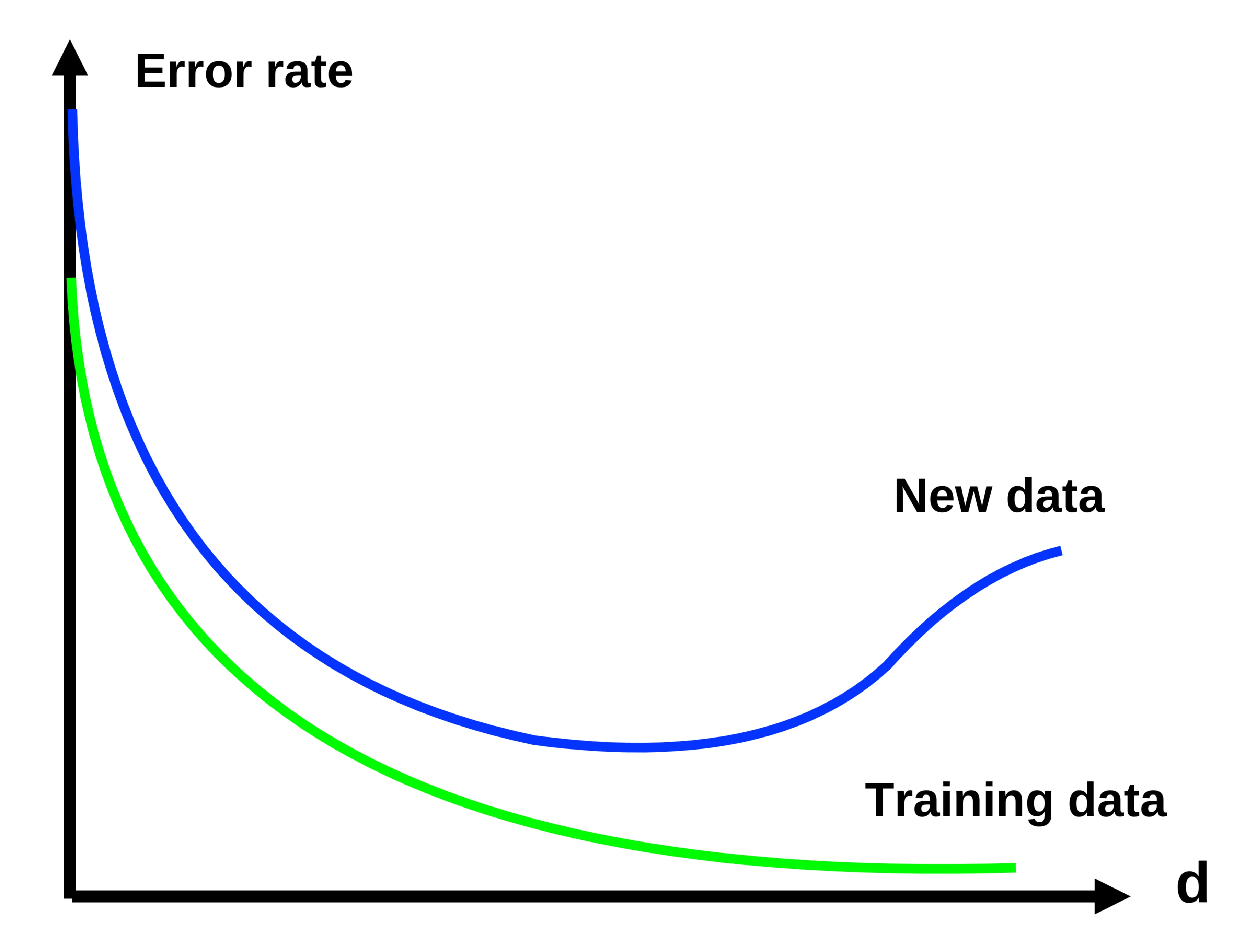
5. The Curse of Dimensionality

The “Curse of Dimensionality” refers to the phenomenon where the performance of a classifier can degrade as the number of features (dimensions, ‘d’) increases, especially if the amount of training data is limited.

• Error Rate: Initially decreases as relevant features are added, but eventually increases as irrelevant or redundant features introduce noise.
• Training Data: The error on the training data typically continues to decrease.
• New Data (Test Data): The error on unseen data (generalization error) starts to increase, indicating overfitting. [[lecture_9_2_featureextraction.pdf#page=6&rect=114,47,637,443|]] The feature vector is represented by: $\vec{x}=\left[\begin{array}{c}{x}_1\\ x_2\\ x_3\\ ...\\ x_d\end{array}\right]$

6. Feature Types (Regional Features)

Several categories of features can be extracted from image regions:

• Color Features: Describe the color distribution within the region.
• Gray Level Features: Based on the intensity values of pixels.
• Shape Features: Quantify the geometric properties of the region.
• Histogram (Texture) Features: Represent the distribution of pixel values or patterns.

Example (Shape Feature): Consider an image with binary region and we want calculate the area. Consider a region with:

• Perimeter: $P$
• Area: $A$

A possible shape feature is circularity: $\frac{P^2}{A}$. This value is dimensionless and provides a measure of how close the shape is to a perfect circle.

7. Moments

Moments are powerful tools for describing the shape and distribution of pixel values within a region.

7.1 Geometric Moments

The geometric moment of order (p, q) is defined as:

$m_{pq}={\int }_{-\infty }^{\infty }{\int }_{-\infty }^{\infty }{x}^p{y}^{q}f(x,y)dxdy\approx {\sum }_i{\sum }_j{i}^p{j}^{q}f[i,j]$

where $f(x,y)$ or $f[i,j]$ is the image intensity function (continuous or discrete).

7.2 Central Moments

Central moments are calculated relative to the centroid (center of mass) of the region, making them translation-invariant:

${\mu }_{pq}={\sum }_i{\sum }_j(i-\tilde{i}{)}^p(j-\tilde{j}{)}^{q}f[i,j]$

where:

• $\tilde{i}=\frac{m_{10}}{m_{00}}$ (x-coordinate of the centroid)
• $\tilde{j}=\frac{m_{01}}{m_{00}}$ (y-coordinate of the centroid)

7.3 Binary Images

For a binary image:

$f[i,j]=\{\begin{array}{ll}1& \text{if }(i,j)\text{ is an object pixel}\\ 0& \text{if }(i,j)\text{ is a background pixel}\end{array}$

• Area: $m_{00}={\sum }_i{\sum }_{j}f[i,j]$ (simply counts the number of object pixels)
• Center of mass: $m_{10}={\sum }_i{\sum }_{j}if[i,j]⟹\tilde{i}=\frac{m_{10}}{m_{00}}$ $m_{01}={\sum }_i{\sum }_{j}jf[i,j]⟹\tilde{j}=\frac{m_{01}}{m_{00}}$

7.4 Moments of Inertia

Central moments can be used to calculate moments of inertia, which describe how the mass (or pixel intensity) is distributed around the centroid:

• ${\mu }_{20}={\sum }_i{\sum }_j(i-\tilde{i}{)}^{2}f[i,j]$
• ${\mu }_{02}={\sum }_i{\sum }_j(j-\tilde{j}{)}^{2}f[i,j]$
• ${\mu }_{11}={\sum }_i{\sum }_j(i-\tilde{i})(j-\tilde{j})f[i,j]$

7.5 Closest Fitting Ellipse

The central moments can be used to define an ellipse that best approximates the shape of the region.

• Orientation: $\theta =\frac{1}{2}{\tan }^{-1}\left(\frac{2{\mu }_{11}}{{\mu }_{20}-{\mu }_{02}}\right)$ (angle of the major axis)

• Eccentricity: $ϵ=\frac{({\mu }_{20}-{\mu }_{02}{)}^2+4{\mu }_{11}^2}{A}$ (measures how elongated the ellipse is)

• Major and Minor Axes:

  • $a^2=\frac{2({\mu }_{20}+{\mu }_{02}+\sqrt{({\mu }_{20}+{\mu }_{02}{)}^2+4{\mu }_{11}^2})}{{\mu }_{00}}$
  • $b^2=\frac{2({\mu }_{20}+{\mu }_{02}-\sqrt{({\mu }_{20}+{\mu }_{02}{)}^2+4{\mu }_{11}^2})}{{\mu }_{00}}$

8. Histogram (Texture) Features

Histograms describe the distribution of pixel values within a region.

• First-order statistics: Relate to the overall distribution of gray levels.
• Second-order statistics: Capture spatial relationships between pixel values (e.g., co-occurrence matrices).

Histogram Calculation:

$P(I)=\frac{\text{Number of pixels with gray level }I}{\text{Total number of pixels in the region}}$

8.1 Moments from Gray Level Histogram

• Moments: $m_p=E\{I^p\}={\sum }_{l=0}^{L-1}{I}^{p}P(I),p=1,2,...$ (where L is the number of gray levels)
• Mean: $m_1=E(I)$ (average gray level)
• Entropy: $H=-E\{\ln P(I)\}=-{\sum }_{l=0}^{L-1}P(I)\ln P(I)$ (measures the randomness or “information content” of the histogram)

8.2 Central Moments from Histogram

${\mu }_p=E\{(I-E(I){)}^p\}={\sum }_{l=0}^{L-1}(I-m_1{)}^{p}P(I),p=1,2,...$

• Variance: ${\mu }_2={\sigma }^2$
• Skewness: ${\mu }_3$ (measures asymmetry)
• Kurtosis: ${\mu }_4$ (measures peakedness)

9. Feature Selection

After generating a large set of potential features, feature selection is crucial.

• Goal: Reduce dimensionality to avoid overfitting and improve computational efficiency.
• Challenges:
  • Exhaustive search (trying all possible combinations) is computationally infeasible.
  • Trial and error can be used, but is not optimal.
• Methods:
  • Suboptimal Search: Heuristic methods like “Branch and Bound”.
  • Linear or Non-linear Mappings: Project the features into a lower-dimensional space (e.g., Fisher’s Linear Discriminant).

Example(Scatter Plot of features) Scatter plot help visualize the separability of classes based on the selected features. Ideally, features should cluster points from the same class together and separate points from different classes.

10. Dimensionality Reduction - Linear Transformations

• Projection: Map high-dimensional feature vectors to a lower-dimensional space.
• Fisher’s Linear Discriminant: Finds a projection that maximizes the separation between classes in a one-dimensional space.