Image Representation & Description

1. Introduction

• Course: CoE4TN4 Image Processing
• Chapter: 11 - Image Representation & Description
• Institution: McMaster University

2. Image Representation & Description: Basics

•  After segmentation, regions are represented and described in a form suitable for computer processing using **descriptors**.
  

• Representing a Region:
  1. External Characteristics: Focus on the boundary. Example: Length of the boundary.
  2. Internal Characteristics: Focus on properties like color and texture.
• Goal: Descriptors should ideally be insensitive to rotation and translation.

3. Chain Code

•  *Definition:* Represents a boundary by a connected sequence of straight-line segments.
  

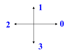
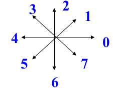
• Uses either 4 or 8 connectivity.

• Method:

  1. Follow the boundary (e.g., clockwise).
  2. Assign a direction code to each segment connecting pixel pairs.

• Direction Codes (Mermaid Diagram):

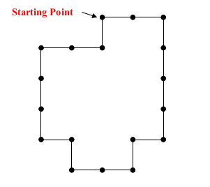Exp: 003333232212111001

• Problems:

  • Dependent on the starting point.
  • Changes with rotation.

• Solutions:

  1. Circular Sequence: Treat the chain code as circular; find the minimum magnitude representation.
  2. First Difference: Count counterclockwise the number of direction changes between adjacent elements.
     • take difference between two consecutive direction number (the latter - the former), and if it is negative, add 4.
     • Example, chain code: $10103322$
     • First difference code: $33133030$

• Shape Number: is the first difference of smallest magnitude.

4. Signature

• Definition: A 1-D functional representation of a boundary.

• Generation Methods:

  • Plot distance from centroid to boundary as a function of angle.

• Example Signatures:

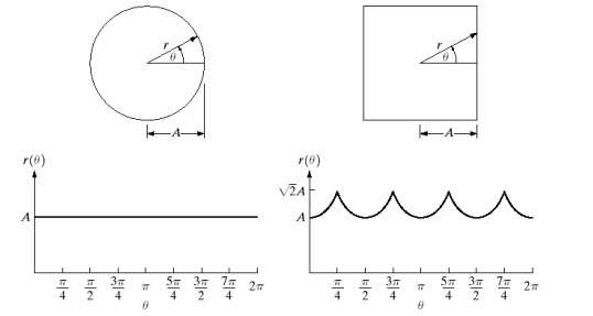
• Other methods can also be used, such as by plotting the angle between the tangent to the boundary at a specific location and a reference line.

• Invariance:

  • Translation: Signatures are inherently invariant to translation.
  • Rotation: Choose a consistent starting point (e.g., farthest from centroid).
  • Scaling: Normalize to a specific range.

• Slope-Density Function: A histogram of tangent-angle values. Peaks correspond to straight segments.

5. Skeletons

• Definition: Represents the structural shape of a region by reducing it to a graph.
• Method: Thinning algorithms (obtain the skeleton).
• Application: Automated inspection.
• Medial Axis Transformation (MAT):
  • For each point p in region R with border B, find the closest neighbor in B.
  • If p has multiple closest neighbors, it belongs to the medial axis (skeleton).
  • Based on the “prairie fire concept.”

6. Simple Boundary Descriptors

• Length: Number of pixels along the contour.
• Diameter: $Diam(B)=\max [D(p_i,p_j)]$, where $p_i$ and $p_j$ are points on the boundary.
• Curvature: Rate of change of slope. (For digital images, difference between slopes of adjacent segments).
• Major Axis: Straight line segment joining the two farthest points on the boundary.
• Minor Axis: Perpendicular to the major axis, forming a bounding box.
• Eccentricity: $\frac{\text{Major Axis}}{\text{Minor Axis}}$
• Basic Rectangle (Bounding Box): Rectangle formed by major and minor axes.

7. Fourier Descriptor

• Given an N-point boundary represented by coordinates: $(x_0,y_0),(x_1,y_1),...,(x_{N-1},y_{N-1})$.

• Represent the boundary coordinates as a complex sequence: $s(k)=x_k+j{y}_k$

• Calculate N point DFT of s(k): $a(u)=\frac{1}{N}{\sum }_{k=0}^{N-1}s(k)\exp (-j2\pi uk/N)$

• $a(u)$ are the Fourier Descriptors.

• By using P of the Fourier descriptors, we can find the following: $\hat{s}(k)={\sum }_{u=0}^{P-1}a(u)\exp (j2\pi uk/N)$

  • If $P<N⟹$ High frequency details of the boundary will be removed.

• Properties:

  • Not directly insensitive to translation, rotation, and scaling.
  • Magnitude of Fourier descriptors is insensitive to rotation.

8. Regional Descriptors

• Area: Number of pixels within a region.
• Compactness: $(\text{Perimeter}{)}^2/\text{Area}$
• Min/Max Gray Levels: Minimum and maximum pixel values in the region.
• Mean and Median Gray Levels: Average and median pixel values.

10. Texture

• Definition: Quantifies smoothness, coarseness, and regularity.
• Approaches:
  1. Statistical: Uses statistical moments of the histogram.
  2. Structural: Uses arrangement of image primitives (texture elements).
  3. Spectral: Based on properties of the Fourier spectrum.

10.1 Statistical Texture

• Moments of Histogram:
  • $n^{th}$ moment: ${\mu }_n(z)={\sum }_{i=0}^{L-1}(z_i-m{)}^{n}p(z_i)$
  • Mean: $m={\sum }_{i=0}^{L-1}{z}_{i}p(z_i)$
  • Variance (Contrast): ${\sigma }^2(z)={\mu }_2(z)$
  • Relative contrast: $R=1-\frac{1}{1+{\sigma }^2(z)}$
  • Third moment (Skewness): ${\mu }_3(z)={\sum }_{i=0}^{L-1}(z_i-m{)}^{3}p(z_i)$
  • Uniformity: $U={\sum }_{i=0}^{L-1}{p}^2(z_i)$ (Maximum when all gray levels are equal)
  • Average Entropy: $e=-{\sum }_{i=0}^{L-1}p(z_i){\log }_{2}p(z_i)$ (Measures variability; zero for a constant image)
• Co-occurrence Matrix
• Histogram-based texture does not take into account relative positions of pixels.
• Let Q be a position operator and G be a $k\times k$ matrix.
• $a_{ij}$ is the number of times that two points with gray levels $z_i$ and $z_j$ occur in a relative position specified by Q.
• Then we define $C=G/n$ as the gray-level co-occurrence matrix, where n is total number of point pairs.
• C depends on Q.

11. Moments

• Moment of order (p+q): $m_{pq}={\sum }_{(x,y)\in R}{x}^p{y}^{q}f(x,y)$
• Central Moments: ${\mu }_{pq}={\sum }_{(x,y)\in R}(x-\bar{x}{)}^p(y-\bar{y}{)}^{q}f(x,y)$
  • Where $\bar{x}=\frac{m_{10}}{m_{00}}$ and $\bar{y}=\frac{m_{01}}{m_{00}}$
• Normalized Central Moments: ${\eta }_{pq}=\frac{{\mu }_{pq}}{{\mu }_{00}^{\gamma }}$, where $\gamma =\frac{p+q}{2}+1$