Image Filtering

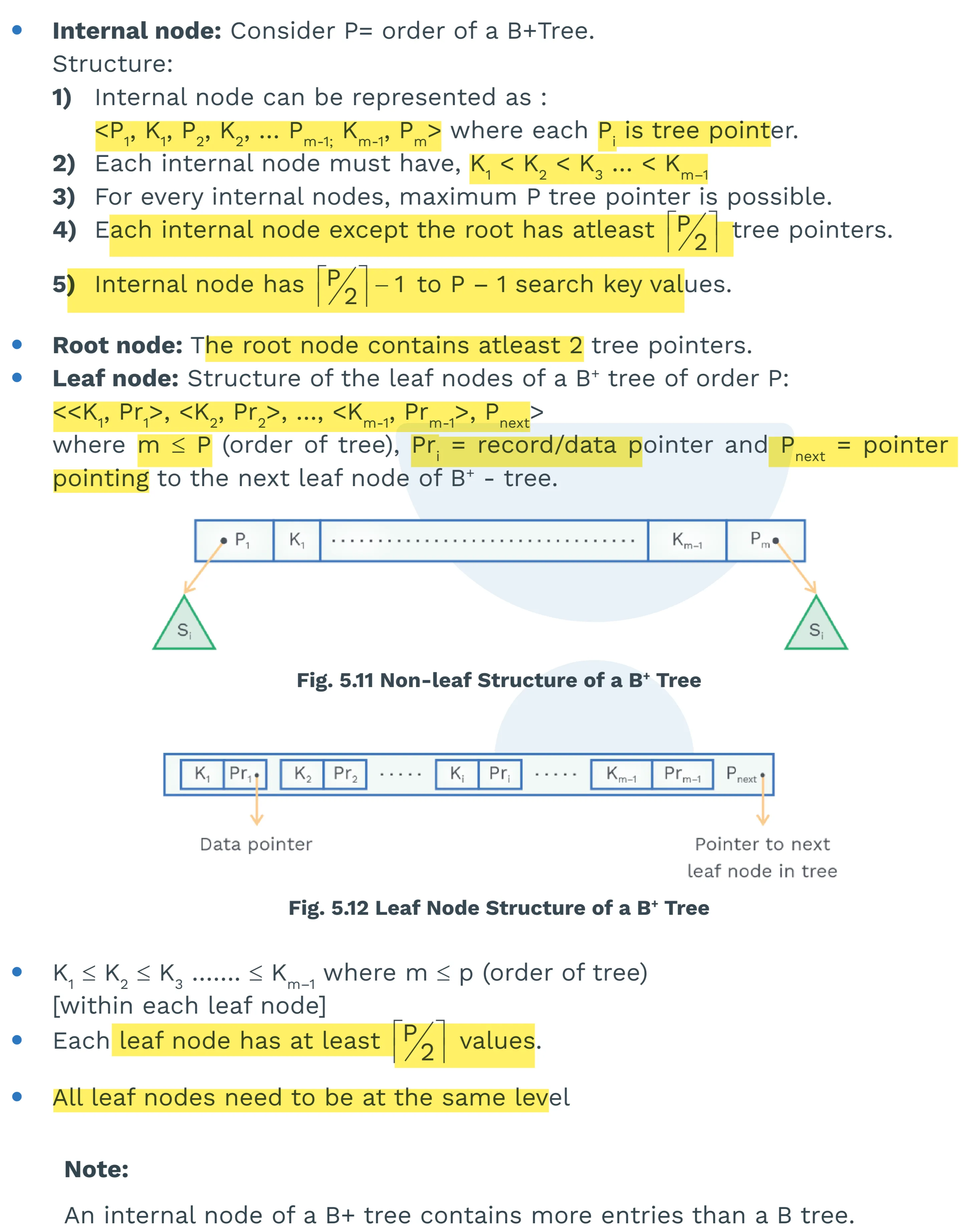
1. Introduction to Filtering

Image filtering modifies an image, often to enhance certain features or remove noise.

Example of simple filtering operations

graph LR
    subgraph Input
    A[1 2 3 4<br>1 2 3 4<br>9 8 3 4<br>1 2 3 4]
    end
    subgraph Filter_F1
    B[1 0 -1<br>1 0 -1<br>1 0 -1]
    end
     subgraph Filter_F2
    C[1<br>1<br>1]
    end
    subgraph Filter_F3
    D[11 12 9 12<br>11 12 9 12]
    end
        subgraph Filter_F4
    E[1 0 -1]
    end

    subgraph Output1
    O1[2 0<br>2 0]
    end
    subgraph Output2
        O2[2 0<br>2 0]
    end
    A -- " " --> B
    A -- " " --> C
   B -- "=" --> O1
 C -- "=" --> D
 D--" "-->E
 E--"="-->O2

2. Edge Detection

Edges represent significant local changes in image intensity. They often correspond to boundaries between objects or regions.

2.1. Detecting Edges with Derivatives

• Concept: Edges are located where the image intensity changes rapidly. Mathematically, this corresponds to high values in the image’s derivative.

• Process:

  1. Take the derivative of the image.
  2. High magnitude values in the derivative indicate edges.

• Discrete Images: Since images are discrete (pixel grids), we use finite differences to approximate derivatives.

Example

graph LR
    subgraph Image
        I
    end
    subgraph "Derivative Filters (fx, fy)"
        F
    end
     subgraph Filtered_Images
        FI
    end

   I -- " " --> F
   F -- " " --> FI

Explanation:

• fx typically represents a filter that calculates the derivative in the horizontal (x) direction.
• fy calculates the derivative in the vertical (y) direction.
• The filtered images show areas of high change in each direction, highlighting edges.

3. Derivative Filters

3.1. Finite Differences

Finite differences are approximations of derivatives for discrete data.

• First-order finite difference (forward difference): $f^{\prime }(x)\approx \frac{f(x+h)-f(x)}{h}$ , where h is a small step (usually 1 pixel). A simplified version for a 1D signal is often represented by the filter: [1, -1](backward) or[-1,1](forward).

• Centered difference: A more accurate representation. The centered differece would look like: [-1, 0, 1]

3.2. Sobel Filter

The Sobel filter is a widely used edge detection filter. It combines a derivative calculation with smoothing.

• Separability: The Sobel filter is separable, meaning it can be implemented as a combination of two 1D filters. This improves computational efficiency.

• Horizontal Sobel Filter (Gx): Detects vertical edges.

  $G_x=\left[\begin{array}{ccc}1& 0& -1\\ 2& 0& -2\\ 1& 0& -1\end{array}\right]=\left[\begin{array}{c}1\\ 2\\ 1\end{array}\right]\ast \left[\begin{array}{ccc}1& 0& -1\end{array}\right]$

  • The [1, 2, 1] part is a smoothing filter (a “tent” filter, similar to a Gaussian).
  • The [1, 0, -1] part is a centered difference derivative.

• Vertical Sobel Filter (Gy): Detects horizontal edges.

  $G_y=\left[\begin{array}{ccc}1& 2& 1\\ 0& 0& 0\\ -1& -2& -1\end{array}\right]=\left[\begin{array}{c}1\\ 0\\ -1\end{array}\right]\ast \left[\begin{array}{ccc}1& 2& 1\end{array}\right]$

• 1D Derivative Filter: [1, 0, -1]

• What is [1,2,1]?: This part is related to smoothing, acts like tent or a triangle, decreasing linearlly from centre to edges.

• Return large responses: This filter would respond strongly to vertical lines because it’s calculating the horizontal gradient. A large change in intensity across the horizontal direction signifies a vertical edge.

3.3. Other Derivative Filters

• Prewitt Filter: Similar to Sobel, but without the central weighting.

  $P_x=\left[\begin{array}{ccc}1& 0& -1\\ 1& 0& -1\\ 1& 0& -1\end{array}\right]$ , $P_y=\left[\begin{array}{ccc}1& 1& 1\\ 0& 0& 0\\ -1& -1& -1\end{array}\right]$

• Scharr Filter: Provides better rotational symmetry than Sobel.

  $S_x=\left[\begin{array}{ccc}3& 0& -3\\ 10& 0& -10\\ 3& 0& -3\end{array}\right]$ , $S_y=\left[\begin{array}{ccc}3& 10& 3\\ 0& 0& 0\\ -3& -10& -3\end{array}\right]$

• Roberts Filter: A simpler, 2x2 filter.

  $R_x=\left[\begin{array}{cc}0& 1\\ -1& 0\end{array}\right]$ , $R_y=\left[\begin{array}{cc}1& 0\\ 0& -1\end{array}\right]$

4. Computing Image Gradients

1. Choose a derivative filter: Select a filter like Sobel (Gx and Gy).

2. Convolve: Convolve the image I with the chosen filters (e.g., $S_x$ and $S_y$). Convolution is a sliding window operation that applies the filter at each pixel.

   $\frac{\partial f}{\partial x}=S_x\ast I$ $\frac{\partial f}{\partial y}=S_y\ast I$

3. Form the Gradient: The gradient is a vector that points in the direction of the greatest intensity change.

   • Gradient Magnitude: Represents the strength of the edge. $||\nabla f||=\sqrt{(\frac{\partial f}{\partial x}{)}^2+(\frac{\partial f}{\partial y}{)}^2}$

   • Gradient Direction: Represents the orientation of the edge. $\theta =ta{n}^{-1}(\frac{\partial f/\partial y}{\partial f/\partial x})$

5. Sobel Edge Detector (Complete Process)

graph LR
    subgraph Input
        Image[Image I]
    end
    subgraph "Sobel Filters"
        Gx[1 0 -1<br>2 0 -2<br>1 0 -1]
        Gy[1 2 1<br>0 0 0<br>-1 -2 -1]
    end
    subgraph "Convolution"
        ConvX["d/dx I"]
        ConvY["d/dy I"]
    end
    subgraph "Gradient Magnitude"
        Grad["sqrt((d/dx I)^2 + (d/dy I)^2)"]
    end
    subgraph Output
        Threshold["Threshold"]
        Edges["Edges"]
    end

    Image -- "*" --> Gx
    Image -- "*" --> Gy
    Gx --> ConvX
    Gy --> ConvY
    ConvX --> Grad
    ConvY --> Grad
    Grad --> Threshold
    Threshold --> Edges

4. Input Image (I): The original image.
5. Sobel Filters (Gx, Gy): The horizontal and vertical Sobel filters.
6. Convolution: The image is convolved with each Sobel filter, producing derivative images in x and y.
7. Gradient Magnitude: The magnitude of the gradient is calculated at each pixel.
8. Thresholding: A threshold is applied to the gradient magnitude. Pixels with magnitudes above the threshold are considered edges.

6. Intensity Profile and Edge Detection

• An edge corresponds to a rapid change in the image intensity function.
• If we plot the intensity along a horizontal scanline, the first derivative will show peaks or valleys at edge locations.
• The second derivative will show zero-crossings at edge locations.

7. Noise and Edge Detection

• Problem: Noise in the image can cause spurious, small variations in intensity, leading to many false edge detections. Derivative filters are very sensitive to noise.

• Solution: Smoothing: Apply a smoothing filter (like a Gaussian blur) before applying the derivative filter. This reduces noise and makes edge detection more robust.

8. Gaussian Smoothing

• Gaussian Filter: A low-pass filter that blurs the image by averaging pixel values, weighted by a Gaussian function.

  $h_{\sigma }(u,v)=\frac{1}{2\pi {\sigma }^2}{e}^{-\frac{u^2+v^2}{2{\sigma }^2}}$

  • $\sigma$ (sigma) controls the amount of smoothing (larger $\sigma$ = more blurring).

The Gaussian Blur is applied first and then the sobel filter is used

9. Derivative of Gaussian (DoG)

• Efficiency: Instead of applying a Gaussian and then a derivative filter, we can combine them into a single filter: the Derivative of Gaussian (DoG).

• Convolution Theorem: The derivative of a convolution is the convolution of the derivative: $\frac{\partial }{\partial x}(h\ast f)=(\frac{\partial }{\partial x}h)\ast f$

  • This means we can take the derivative of the Gaussian filter first, and then convolve that with the image.

10. Laplacian of Gaussian (LoG)

• Second Derivative: The Laplacian is a second-order derivative operator. It highlights regions of rapid intensity change.

• Laplacian Filter (1D): A simple 1D Laplacian filter is [1, -2, 1]. Approximating 2nd order finite difference. $f^{\prime \prime }(x)=li{m}_{h->0}\frac{f(x+h)-2f(x)+f(x-h)}{h^2}$

• Laplacian of Gaussian (LoG): Combine Gaussian smoothing with the Laplacian:

  1. Smooth the image with a Gaussian: $\tilde{S}=g\ast \tilde{I}$
  2. Apply the Laplacian: ${\Delta }^{2}S=\frac{{\partial }^2}{\partial x^2}S+\frac{{\partial }^2}{\partial y^2}S$
  3. Find zero crossing.

• Zero-Crossings: Edges are located at the zero-crossings of the LoG output.

• Four cases of Zero Crossings: {+,-},{+,0,-},{-,-},{-,0,+}.

• Slope of Zero Crossings: {a,-b} is |a+b|.

• Advantages: LoG is less sensitive to noise than a simple Laplacian, and zero-crossings provide precise edge localization.

• Disadvantage: LoG is still susceptible to noise and, can cause spurious edges detected.

11. 2D Gaussian, DoG, and LoG (Visualized)

graph LR
    subgraph Gaussian
    A[Gaussian]
    end
    subgraph "Derivative of Gaussian"
      B[Derivative of Gaussian]
    end
    subgraph "Laplacian of Gaussian"
       C[Laplacian of Gaussian]
    end

• Gaussian: A bell-shaped curve.
• DoG: Looks like a “Mexican hat” (a positive peak surrounded by a negative region).
• LoG: Also has a characteristic shape with positive and negative regions.

This comprehensive breakdown covers all the key concepts and equations from the provided slides, making it a suitable resource for digital notes. The MathJax formatting ensures correct mathematical representation, and the Mermaid diagrams provide visual aids where appropriate.