Computer Vision - Texture

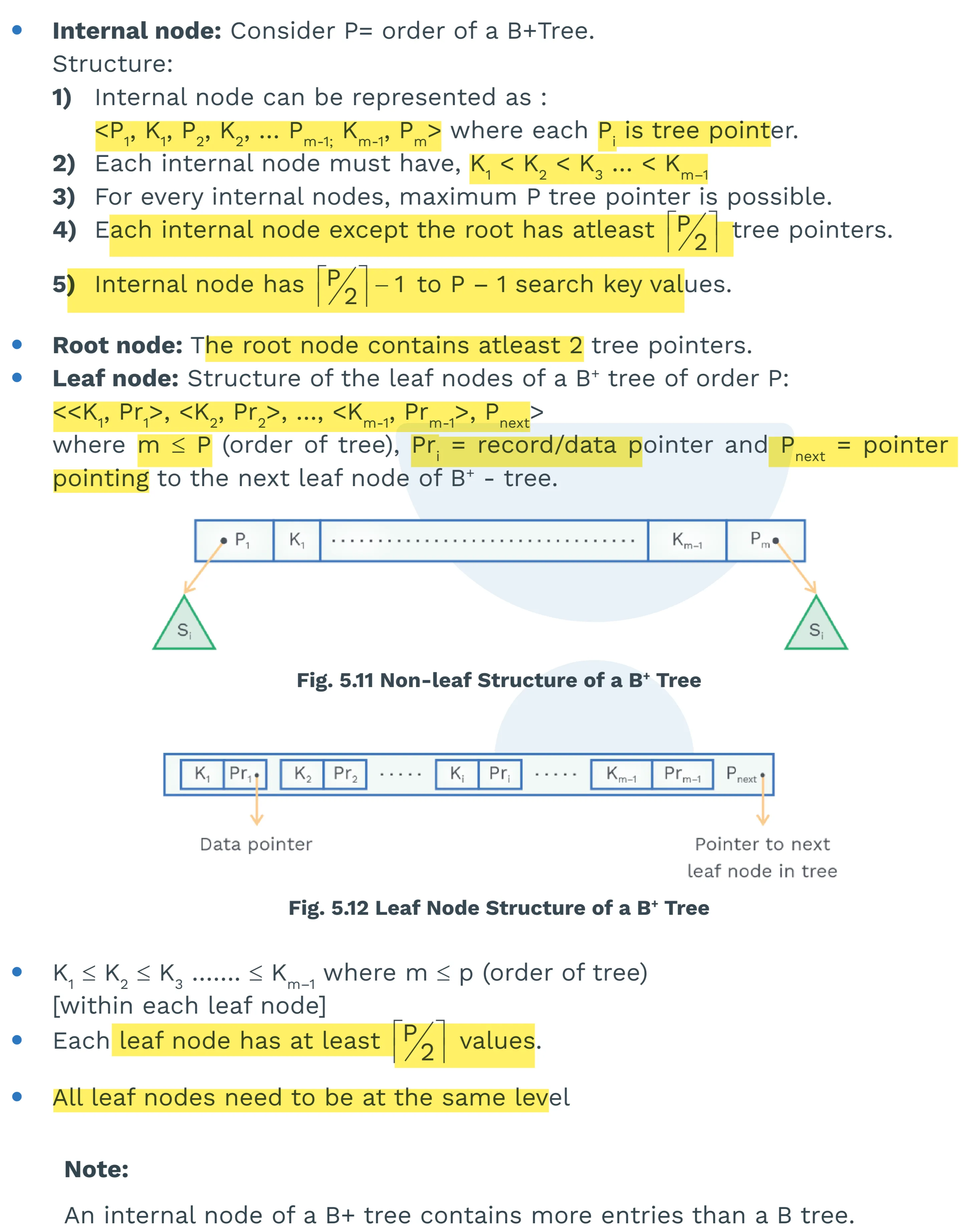
2. What is Texture?

• Definition: Texture is easy to recognize visually but difficult to define precisely. It generally refers to:
  • Views of a large number of small objects (e.g., grass, foliage, pebbles).
  • Surfaces exhibiting patterns (e.g., spots, stripes, wood grain, skin).
• Key Characteristics: Texture consists of organized patterns of regular sub-elements.
• Scale Dependence: Whether a visual pattern is considered “texture” depends on the scale at which it’s viewed. A single leaf is not texture, but a field of leaves is.

3. Texture-Related Problems

Several computer vision tasks involve texture:

• Texture Analysis: Representing and modeling texture. The goal is to find a mathematical description of a texture.
• Texture Segmentation: Dividing an image into regions where the texture is consistent. This is like object segmentation, but based on texture instead of, say, color.
• Texture Synthesis: Generating large areas of texture from small example patches. Think of this like “texture cloning.”
• Shape from Texture: Inferring the 3D shape or orientation of a surface from the texture in the image. Texture gradients (changes in texture) provide cues about surface orientation.

4. Representing Texture: Textons

• The Goal: To represent texture, we look for the regular sub-elements that compose it. These sub-elements are sometimes called “textons.”
• Approach:
  1. Find the sub-elements: Identify the repeating patterns.
  2. Represent their statistics: Describe the characteristics of the sub-elements (e.g., size, shape, orientation).
  3. Reason about their spatial layout: How are the sub-elements arranged relative to each other?
• Challenge: There is no universally agreed-upon, definitive set of textons.

5. Texture Analysis Approaches

Several approaches are used for texture analysis:

• Co-occurrence Matrices (Classical): A statistical method based on the spatial relationships between pixel intensities.
• Spatial Filtering: Applying filters (like edge detectors or Gabor filters) to extract texture features.
• Random Field Models: Statistical models that describe the probability of pixel values given their neighbors. (Not covered in detail in these slides).

6. Co-occurrence Matrix Features

• Objective: To capture the spatial relationships between pixel intensities in a texture.

• Co-occurrence Matrix (C): A 2D array where:

  • Rows and columns represent the possible image intensity values.
  • $C_d(i,j)$ counts how many times intensity value i occurs next to intensity value j with a specific spatial relationship d.
  • The spatial relationship d is defined by a vector $d=(dr,dc)$, representing the offset in rows (dr) and columns (dc) between the two pixels.

Example:

Consider a small grayscale image and a displacement vector $d=(3,1)$:

1 1 0 0
1 1 0 0
0 0 2 2
0 0 2 2
0 0 2 2
0 0 2 2

The co-occurrence matrix $C_d$ would be:

   0 1 2
0 [1 0 3]
1 [2 0 2]
2 [0 0 1]

• Normalized Co-occurrence Matrix ($N_d$): Each entry in $C_d$ divided by sum of entire matrix. This makes co-occurrence statistics less sensitive to number of pixels.

• Quantitative Features from Co-occurrence Matrices:

  • Energy: $Energy={\sum }_i{\sum }_j{N}_d(i,j{)}^2$ (Measures uniformity. Higher for homogeneous textures.)
  • Entropy: $Entropy=-{\sum }_i{\sum }_j{N}_d(i,j){\log }_2{N}_d(i,j)$ (Measures disorder. Higher for more random textures.)
  • Contrast: $Contrast={\sum }_i{\sum }_j(i-j{)}^2{N}_d(i,j)$ (Measures local variations. Higher for textures with large intensity differences.)
  • Homogeneity: $Homogeneity={\sum }_i{\sum }_j\frac{N_d(i,j)}{1+|i-j|}$ (Measures similarity. Higher for textures with similar pixel values.)
  • Correlation: $Correlation=\frac{{\sum }_i{\sum }_j(i-{\mu }_i)(j-{\mu }_j)N_d(i,j)}{{\sigma }_i{\sigma }_j}$ (Measures linear dependencies. ${\mu }_i$, ${\mu }_j$ are means, and ${\sigma }_i$, ${\sigma }_j$ are standard deviations of rows and columns.)

• Disadvantages of Co-occurrence Matrices:

  • Computationally expensive, especially for large images and many intensity levels.
  • Sensitive to grayscale distortion (since they directly depend on pixel values).
  • More suitable for fine-grained textures than for textures with large-scale structures.

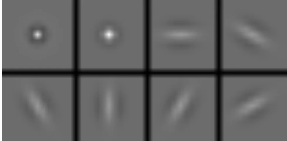
7. Spatial Filtering Approaches

• Core Idea: Apply filters to the image to detect the “sub-elements” of the texture.
• Filter Responses: The magnitude of the filter response indicates the presence of a particular texture element.
• Common Filter Types:
  • “Spot” filters: Gaussians or weighted sums of concentric Gaussians. These detect blob-like features.
  • “Bar” filters: Differencing oriented Gaussians. These detect edges or lines at specific orientations.

Example Filters (visual representation):

Texture, p.7